ECE 445S Laboratory: Week 1
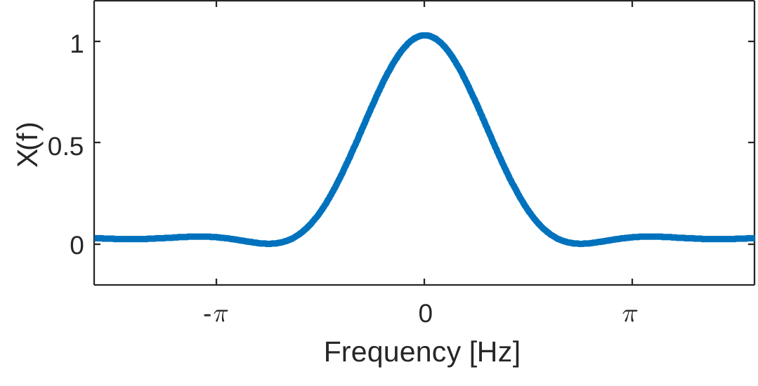
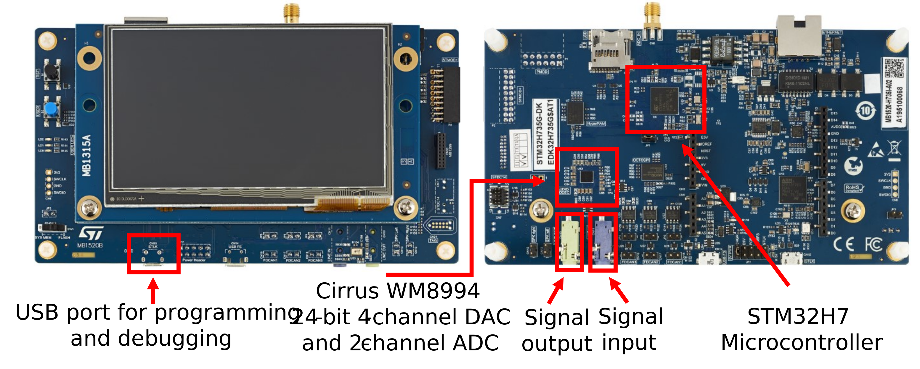
Hardware Overview
C Programming
- Data types
- Pointers
- Functions
- Arrays
- For loops
Data Types
- C language does not provide exact rules for data types
- Example:
int- Must be at least 16 bits, but can be larger
- Must include the range [−32,767, +32,767]. Often, -32,768 is included as well.
- Example:
- Toolchain used in lab provides exact specifications for data types
int16_t16-bit signed integeruint32_t32 bit unsigned integerfloat32_t32 bit (single precision) floating point
Pointers and functions
Example: measuring clock cycles
uint32_t* systick = (uint32_t*) 0xe000e018;
void tic(void)
{
    t = *systick;
}
uint32_t toc(void)
{
    return t - *systick;
}
Arrays and for loops
- Example: cosine lookup table
int16_t table[16];
float32_t amplitude;
flat32_t omega0 = 0.0576;

for (uint32_t n = 0; n < 16; n+=1)
{
    amplitude = arm_sin_f32(n * omega0);
    table[n] = OUTPUT_SCALE_FACTOR * amplitude;
}
Linear vs circular buffer
Example: Shift all elements of an $N=16$ element array and add a new element to the start.
Circular buffer
float32_t x[16] = {0};
int32_t position = 0;
     .
     .
     .
void circular_buffer_shift(float32_t new_element)
{
    position = (position-1) % 16
    x[position] = new_element
}
MATLAB
Data Types in MATLAB
- By default, every variable in MATLAB is a 2d array of double precision floating point values
- To use another datatype, call the corresponding function (
single(),int16(),uint32(), etc) - View the size and type of variables using the
whos()function - By default
iandjrepresent $\sqrt{(-1)}$. Be careful naming variables that overwrite these! - Data automatically become complex if any multiple of
jis added, e.g.1-3j
Vector and array operations
- You can use for loops to perform vector and array operations
- Most of the time, there is an easier and more computationally efficient way
A = [1,2,3
     4,5,6];
B = [7,8,9
     3,2,1];
Element-wise product of two matrices using for loops
for i_row = 1:2
    for i_col = 1:3
        C(i_row,i_col) = A(i_row,i_col) * B(i_row,i_col);
    end
end
Vector and array operations
A = [1,2,3
     4,5,6];
B = [7,8,9
     3,2,1];
element-wise product of two matrices using .* operator
C = A .* B;
Matrix-matrix product using * operator and ' for transpose.
C = A * B';
Creating plots
- To describe your plot to MATLAB, give the
plot()function the (x,y) coordinates of each point you want to plot - Put all of the x coordinates in a vector and the y coordinates in a second vector
- Use
plot(x,y)to represent continuous signals - Use
stem(x,y)to represent discrete signals - Call the
figure()function before a plot to put it in a new window - Use
hold on;to overlay on the previous plot - Use the incantation
set(0,'DefaultFigureWindowStyle','Docked')to keep all figures in the same window but make an new tab for each
Floating point
- Integer and other fixed-point data types have the same spacing between all possible values
- Useful for representing natural numbers or the value read from ADC
- Distance between adjacent floating point numbers is variable
- Useful for representing filter coefficients
- Less build up of error for sequences of operations compared to fixed point
- Single precision (near 1.0) is roughly equivalent to 8 decimal points
- Largest possible value is about $3.4 \times 10^{38}$
- Near zero, the smallest distance between values is about $1.4\times 10^{-45}$
Linear Systems and Signals
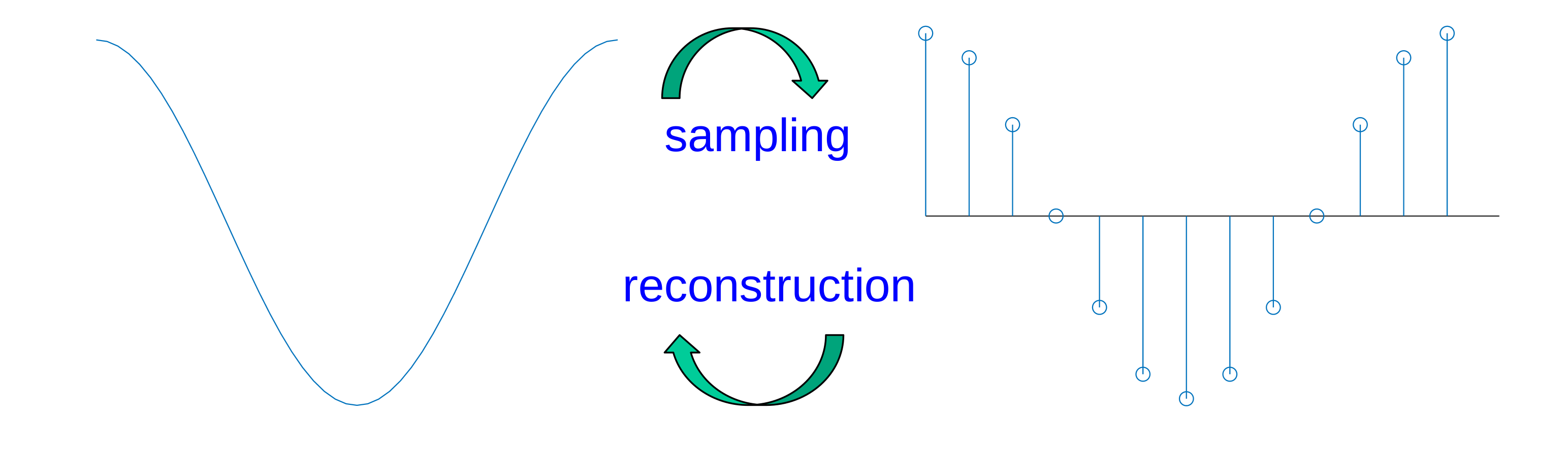
Sampling and Reconstruction
- Sampling (continuous-time to discrete-time conversion)
- $x[n] = x(n T_s)$
- Reconstruction (discrete-time to continuous-time conversion)
- A continuous-time signal $x(t)$ with frequencies no higher than $f_{\text{max}}$ can be reconstructed exactly from its samples $x[n] = x(n T_s)$ if samples are taken at a sampling rate $f_s > 2f_{\text{max}}$
Transforms
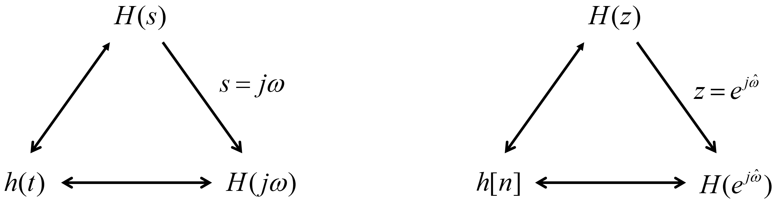
Preview of the different transforms we will use in this class:
- Laplace transform
- Z-transform
- Fourier transform
- Discrete-time Fourier transform (DTFT)
- Fourier series
- Discrete Fourier transform (DFT, a.k.a FFT)
All of these have certain properties in common (with a few caveats)
- $ \text{Multiplication} \leftrightarrow \text{Convolution} $
- $ \text{Stretch} \leftrightarrow \text{Contract}$
Transforms
Fourier transform example
What is the fourier transform of $ x(t) = \left(1+\cos(2\pi t)\right) \left( \text{rect}(t) \right)$ ?
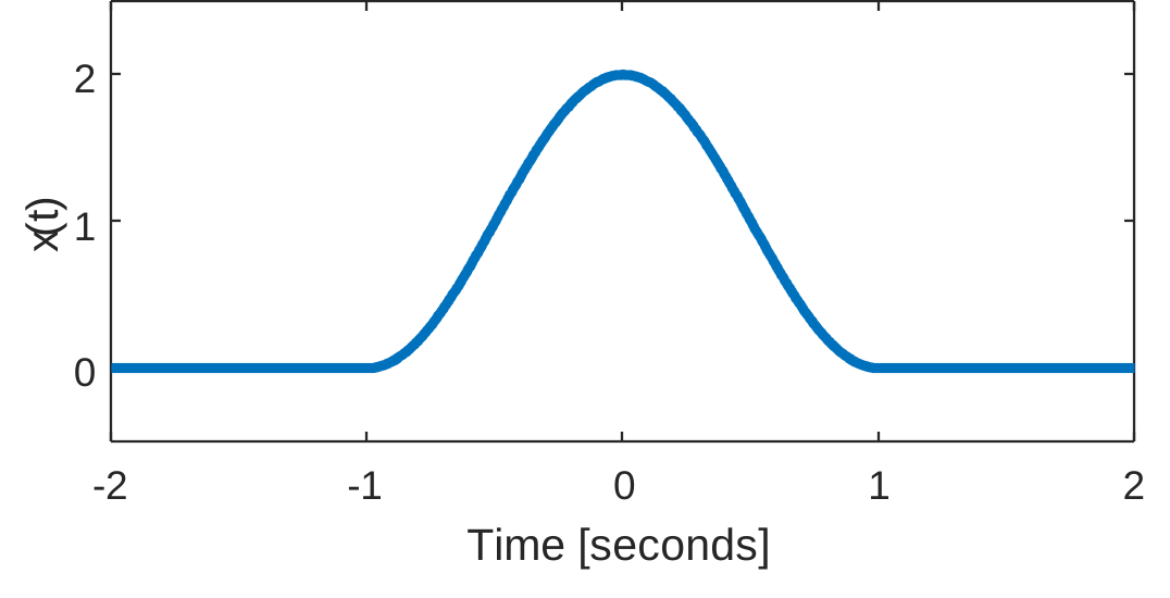
Fourier transform example
The Fourier transform of a constant $1$ is $\delta(f)$.
The Fourier transform of $ \cos(at) $ is $\frac{1}{2}\left[ \delta(f-\frac{a}{2\pi}) + \delta(f+\frac{a}{2\pi}) \right]$
The Fourier transform of $ \text{rect} (t) $ is $\text{sinc}(f)=\frac{\sin(\pi f)}{\pi f}$
Multiplication in time domain is convolution in frequency domain
Sifting property: $f(t) * \delta(t-t_0) = f(t-t_0)$
Fourier transform example